Machine Learning (Part 3)
Table of contents
- Overview
- From Averages to Weighted Sums
- Perceptrons
- Learning From Mistakes
- Putting It All Together
- Results
- From Perceptrons to Neural Networks
- Computational Requirements
- Working in Machine Learning
- Optional Reading: QuickDraw
Overview
In parts 1 and 2, we built a simple image classifier using the nearest prototype approach. We started with a naive solution that used a single feature (average pixel value) and then improved it by using all pixel values. However, the classifier’s performance was still limited (about \(82\%\) accuracy).
In this lesson, we will introduce a well-known technique inspired by how neurons in the brain process information. While our discussion will be simplified, it will give you a glimpse into the ideas behind neural networks, which are widely used in modern machine learning systems (including ChatGPT).
From Averages to Weighted Sums
Before we proceed, let’s revisit the concept of sums and averages and see how they relate.
The Average Revisited
In part 1, we computed the average pixel value of an image by summing all pixel values and dividing by the number of pixels. This means that we gave equal importance (weight) to all pixel values when computing the average.
Mathematically, given a set of values \(x_0, x_1, ..., x_{n-1}\), the average is computed as follows:
\[\text{Average} = \frac{x_0 + x_1 + ... + x_{n-1}}{n}\ =\ (\tfrac{1}{n}\times x_0)\ +\ (\tfrac{1}{n}\times x_1)\ +\ ...\ +\ (\tfrac{1}{n}\times x_{n-1})\]DEFINITION
An average is a special case of a more general concept called a weighted sum. In a weighted sum, we assign a weight to each value when combining them. When all weights are equal (e.g., \(\tfrac{1}{n}\)) and sum up to 1, the weighted sum is the average.
Using Weights
In many situations, treating all values equally does not make sense. Some values should have more influence than others.
For example, suppose we have three exam scores:
Quiz = 100
Midterm Exam = 90
Final Exam = 50
If we compute a weighted sum where every score has the same weight \(\tfrac{1}{3}\), we obtain the ordinary average:
\[(\tfrac{1}{3}\times 100)\ +\ (\tfrac{1}{3}\times 90)\ +\ (\tfrac{1}{3}\times 50)\ =\ 80\]However, we know that the midterm exam is more important than the quiz and the final exam is more important than the midterm. To reflect this, we can assign weights to each score:
- Quiz weight = 0.2
- Midterm weight = 0.3
- Final Exam weight = 0.5
Using these weights, we compute:
\[(0.2 \times 100) + (0.3 \times 90) + (0.5 \times 50) = 72\]This is a better reflection of the student’s performance.
DEFINITION
Given a set of values \(x_0, x_1, ..., x_{n-1}\) and their corresponding weights \(w_0, w_1, ..., w_{n-1}\), the weighted sum is computed as follows:
\[\text{Weighted Sum} = (w_0 \times x_0) + (w_1 \times x_1) + ... + (w_{n-1} \times x_{n-1})\]
Here is a simple Python function to compute the weighted sum:
def weighted_sum(values, weights):
    total = 0
    for i in range(len(values)):
        total += values[i] * weights[i]
    return total
Perceptrons
Overview
Now that we understand weighted sums, we can introduce a simple model called the perceptron.
A perceptron for the digit 0 is a predictor that takes in an image (represented as a 1D list of pixel values) and produces a score that indicates how likely the image is to be the digit 0.
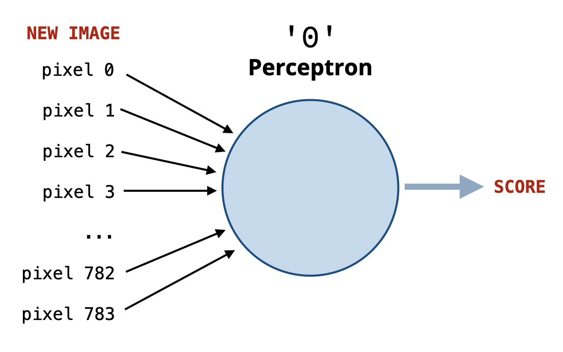
The higher the positive score, the more confident the perceptron is that the image is a 0. The lower (more negative) the score, the more confident it is that the image is not a 0.
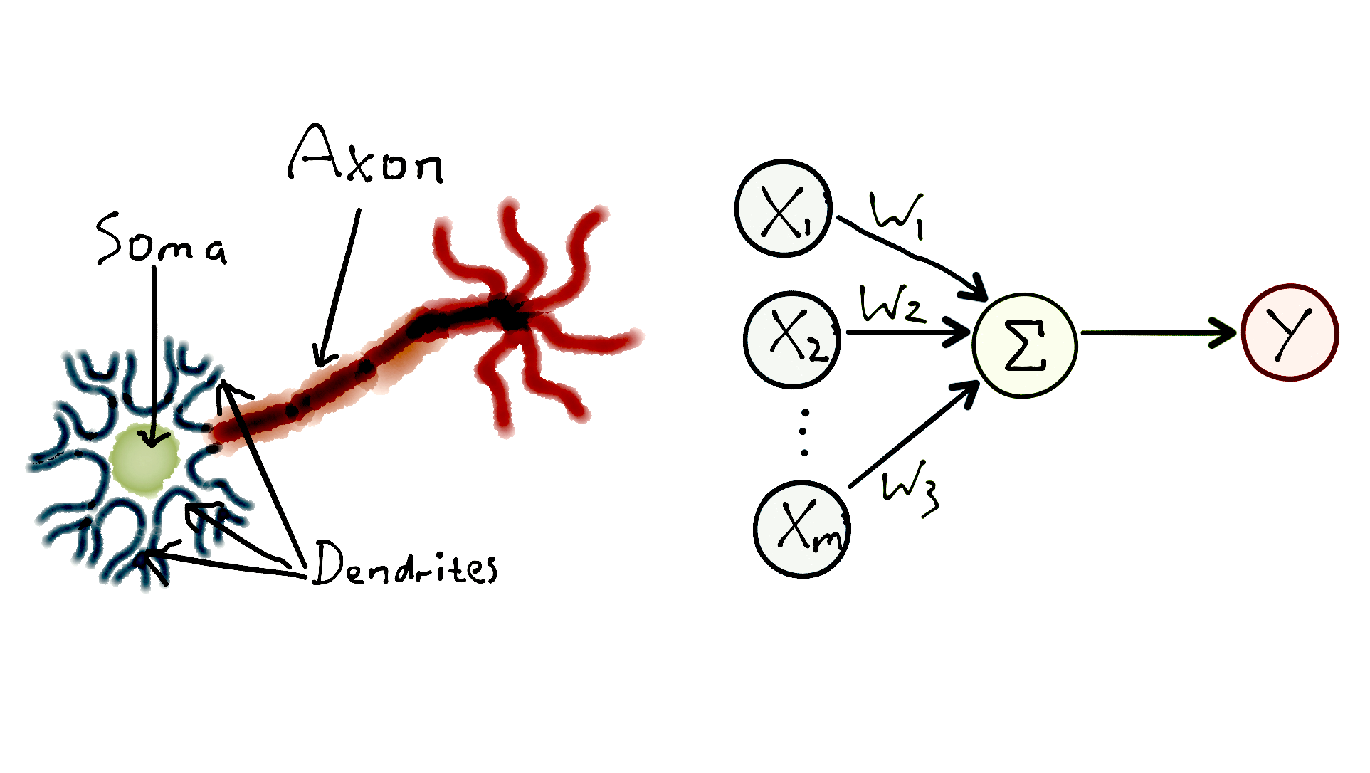
A perceptron is analogous to a biological neuron in the brain, which receives signals from other neurons. If the combination of these signals is strong enough, the neuron gets activated and sends a signal to other neurons.
Perceptron Implementation
What inputs does the perceptron take? And how does it compute the score?
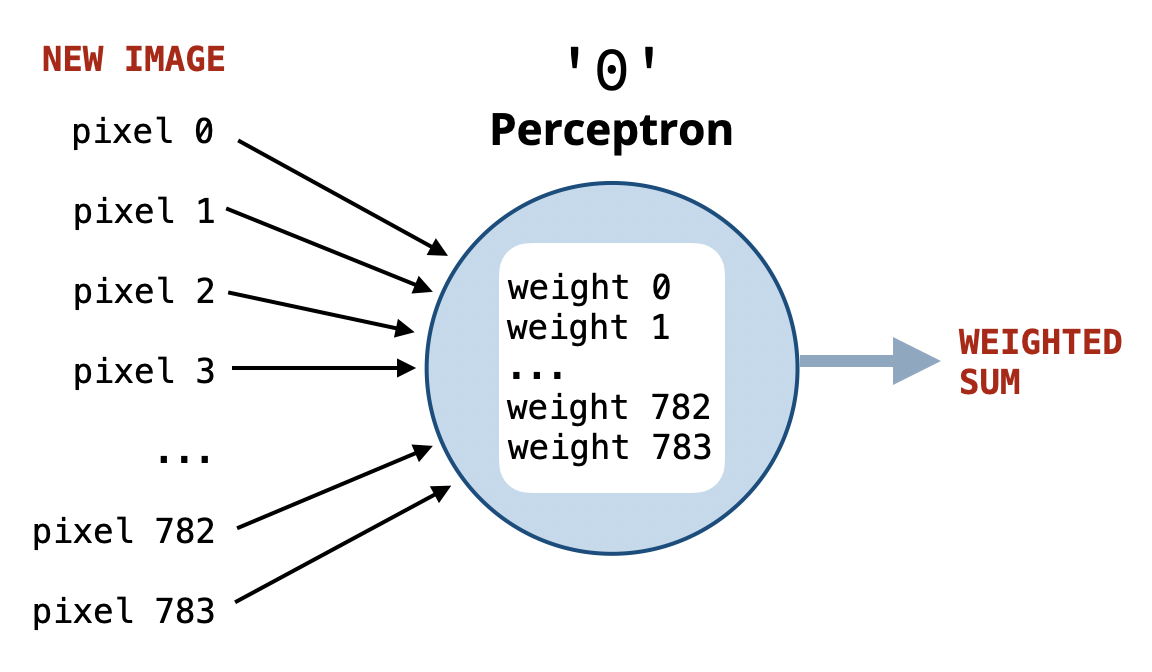
Suppose someone gives us a function named get_weights that returns a list of weights representing the importance of each pixel for recognizing the digit 0, where:
- Important pixels have positive weights.
- Unimportant pixels have negative weights.
Using such weights, we can implement the perceptron for digit 0 simply by computing the weighted sum of the pixel values using these weights.
Examples
Assume we have the following (hypothetical) weights for a perceptron for digit 0:
[10, 15, 20, 23, 15, 5, 30, ..., -5, -10, -8, -12, -33, -20]
  first half: +ve weights        second half: -ve weights
Assume that we have two images represented as 1D lists of pixel values:
Image A (digit 0): [255, 255, 255, 255, 255, 255, 255, ..., 0, 0, 0, 0, 0, 0]
Image B (digit 1): [0, 0, 0, 0, 0, 0, 0, ..., 255, 255, 255, 255, 255, 255]
Which image is more likely a 0 (according to the perceptron for digit 0)?.
We compute the scores for both images:
score_A =   10     15     20     ...  -5  -10  -8
         x  255    255    255    ...   0   0   0
            ------------------------------------------
         =  2550 + 3825 + 5100 + ... + 0 + 0 + 0
            large positive score (image A is likely a '0')


score_B =   10     15     20     ...  -5   -10   -8
         x   0      0      0     ... 255   255   255
            ------------------------------------------
         =   0 +    0 +    0 + ... -1275 -2550 -2040
            large negative score (image B is unlikely a '0')
Classifying Any Digit
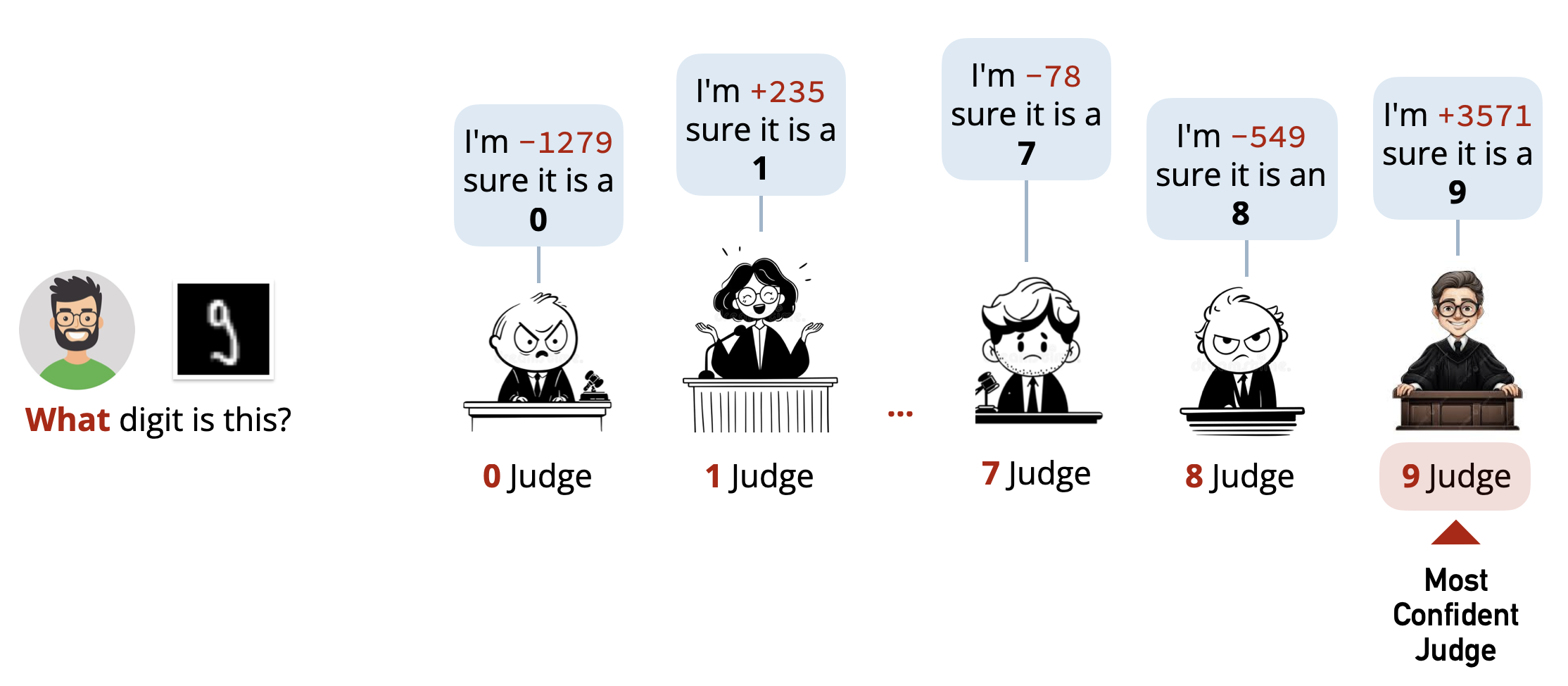
To be able to classify any digit, we need a perceptron for each digit \((0-9)\). Each perceptron will act as a judge or expert that evaluates whether the input image corresponds to its digit or not. The digit with the highest positive score will be our final prediction.
Implementation
Here is how we can implement the multi-perceptron classifier:
- We need a function
get_weightsthat returns the weights for a single digit. - We need a function
get_all_weightsthat returns the weights for all digits. - We need a function
predictthat does the following:- For each digit, compute the score (weighted sum).
- Keep track of the digit with the highest score.
- Return that digit as the prediction.
def get_weights(folder):
    # We don't know yet how to implement this function!
    pass


# For every digit, get a list of weights
# Return a list of lists of weights:
# [
#  [weights for digit 0],
#  [weights for digit 1],
#   ...,
#  [weights for digit 9]
# ]
def get_all_weights(training_folder):
    all_weights = []
    for digit in range(10):
        folder = training_folder + '/' + str(digit)
        weights = get_weights(folder)
        all_weights.append(weights)
    return all_weights

def predict(pixels, all_weights):
    result = None
    max_score = None

    # Loop over each digit, compute its score,
    # and keep track of the max
    for digit in range(10):
        score = weighted_sum(pixels, all_weights[digit])
        if max_score is None or score > max_score:
            max_score = score
            result = digit

    return result
This is our multi-perceptron classifier! The only missing piece is how to compute the weights for each digit in the get_weights function.
Learning From Mistakes
To compute the weights for each digit, we can use a simple learning algorithm inspired by how biological neurons adjust their connections based on experience.
Let’s consider how to train the perceptron for digit 0 using a set of training images.
1. We’ll start with all weights initialized to zero. This is equivalent to having no knowledge about which pixels are important.
If we use these weights to predict the digit in an image, the score will always be zero, and the perceptron will not be able to make any meaningful predictions.
2. Next, we will go through each image in the training set for digit 0 and make a prediction using the current weights. This leads to one of the following cases:
Case 1: True Positive (Image is
0, Score> 0,CORRECTPrediction):
We don’t need to change the weights since they are already working well for this image.Case 2: True Negative (Image is not
0, Score<= 0,CORRECTPrediction):
Nothing needs to be changed here either.Case 3: False Negative (Image is
0, Score<= 0,INCORRECTPrediction):
This is a mistake! The perceptron did not produce a positive score. To fix this, we will increase the weights for the pixels that are white (high pixel values) in this image. This will make it more likely for similar images to produce a positive score in the future.Case 4: False Positive (Image is not
0, Score> 0,INCORRECTPrediction):
This is also a mistake! The perceptron produced a positive score for a non-0image. To fix this, we will decrease the weights for the pixels that are white (high pixel values) in this image to make it less likely for similar images to produce a positive score in the future.
By repeating this process for all images in the training set, the perceptron will gradually learn which pixels are important for recognizing the digit 0 and adjust its weights accordingly.
To see how this training process works, try the following interactive simulation:
Interactive Demo: Train Your Own Perceptron →
Watch a neuron learn to recognize digits in real time.
Putting It All Together
Now we have an idea about how to compute the weights for each digit and implement the get_weights function.
However, we will skip doing that and will provide you with a complete implementation as an optional reading. The implementation uses more details to make the learning process more effective. For example:
Learning Epochs.
It uses multiple learning epochs, where each epoch goes through all the training images once. The learning process is repeated for multiple epochs to improve the weights further.Other Optimizations.
It learns from the training set in random order during each epoch to avoid biasing the learning process. It also preloads all images into memory to speed up the learning process, and normalizes pixel values to be between \(0\) and \(1\) instead of \(0\) and \(255\), in addition to a few other optimizations.
You don’t have to worry about these details now. It is enough to understand the main idea behind how a perceptron is trained and how it makes predictions.
Results
Using the above perceptron implementation, we achieve a test accuracy of about:
\[88.75\%\]This is a significant improvement over our previous nearest prototype classifier (about \(82\%\) accuracy).
Is this the best we can do? Not quite! People have achieved much higher accuracy (over \(99\%\)) on this dataset using more advanced techniques.
From Perceptrons to Neural Networks
Our solution uses multiple perceptrons (one for each digit) working independently. However, would you call a brain that consists of only 10 neurons (one for each digit) intelligent? Probably not!
Our brain contains a massive network of neurons working together. Similarly, many real-world classification systems are built using Neural Networks, which consist of many perceptrons connected together.
In a Neural Network, perceptrons are organized into multiple layers, where the output of one layer serves as the input to the next layer. In such a setup, the result is not computed simply by taking the maximum score among perceptrons, but rather through a series of transformations across layers.
Larger neural networks with many layers (called deep neural networks) have been shown to achieve remarkable performance on various tasks, including image recognition, natural language processing, and game playing. They are the backbone of many modern AI systems including “Large Language Models” (LLMs) like ChatGPT.
Computational Requirements
Training a single perceptron for one digit using the above implementation requires going through all the \(6,000\) training images. This is repeated for all \(10\) digits, and for multiple epochs (e.g., \(10\) epochs).
If you run the code, you’ll notice that it is slow. Imagine applying this to another problem where:
The input images are larger (e.g., \(800 \times 600\) pixels instead of \(28 \times 28\)).
The dataset is larger (e.g., millions of images instead of thousands).
The model is more complex (e.g., thousands of perceptrons instead of just \(10\)).
In such cases, training the model could take days or even weeks on a regular computer. This is one of the main challenges in machine learning, and it has led to the development of specialized hardware (like GPUs) and optimization techniques to speed up the training process.
Can you imagine how much time, data, and computational power it takes to train something like ChatGPT?
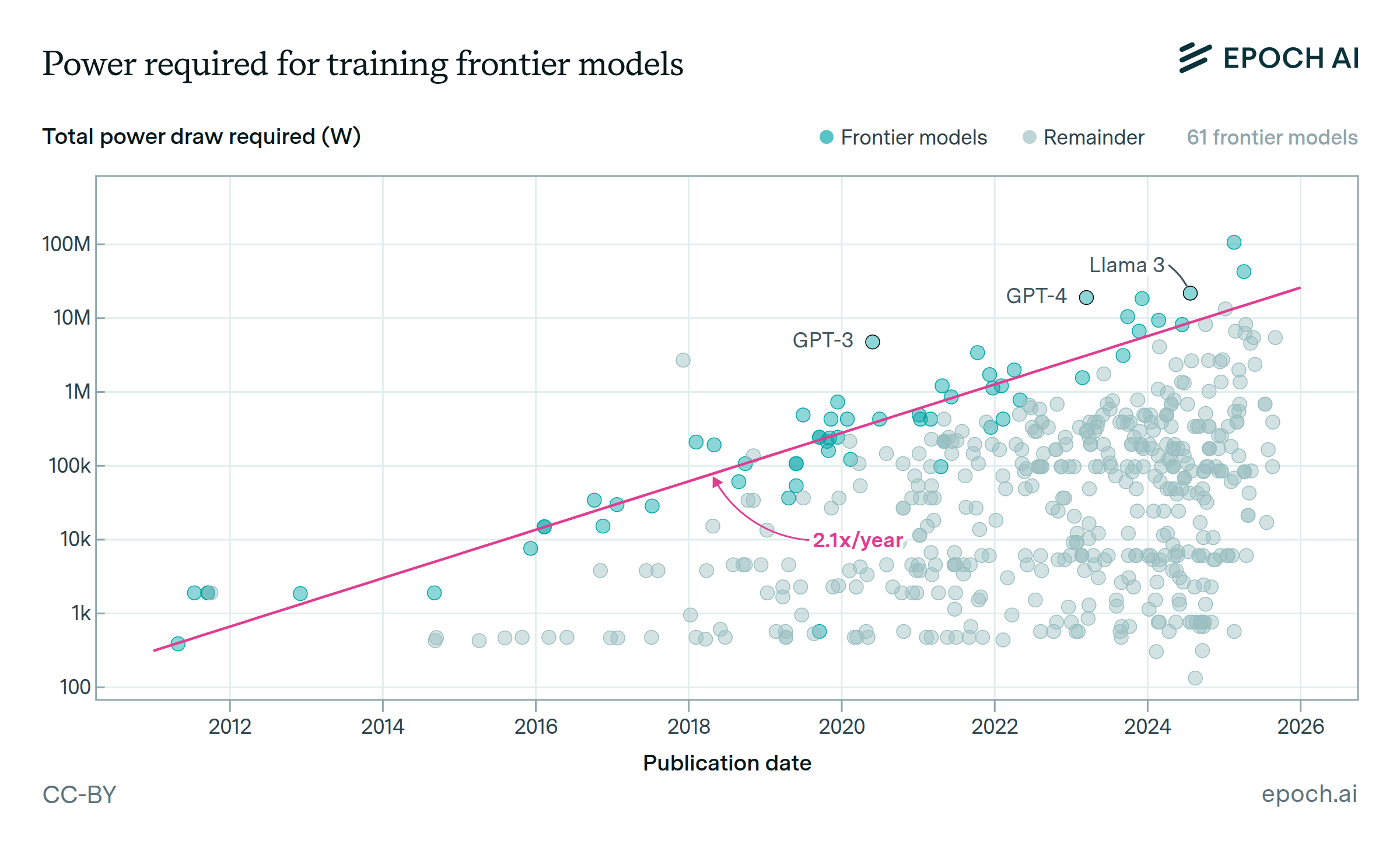
The chart above shows how much electrical power (in megawatts) is consumed by training various AI models over the years.
For context, a single megawatt (MW) can power hundreds of homes. Therefore, the 100 Megawatts (MW) needed to train Grok3 can supply tens of thousands of residences, depending on local usage patterns.
Working in Machine Learning
By now, you should have a basic understanding of what it takes to build a machine learning system. If you work as a data scientist or machine learning engineer, you will often find yourself doing one or all of the following tasks:
Data Preparation.
Collecting, cleaning, and organizing data to be used for training and testing machine learning models. The data we used in this lesson was already prepared for us, but in real-world scenarios, this step can be time-consuming and complex.Model Development, Training, and Evaluation.
Designing and implementing machine learning models (like the perceptron) to solve specific problems. This involves extracting features from data, selecting and adapting appropriate algorithms, tuning parameters, assessing performance, and iterating to improve results.Deployment.
Integrating trained models into applications or systems for real-world use.
Optional Reading: QuickDraw
Creating good datasets for training machine learning models can be challenging. One interesting approach to collecting large datasets is through games.
QuickDraw is an online game developed by Google that collects doodles drawn by users worldwide. Players are prompted to draw a specific object (e.g., “cat”, “house”, “car”) within a time limit. The game uses machine learning to guess what the player is drawing based on the doodle.
Check the dataset collected from QuickDraw here →
You can contribute to the dataset by playing the game or help clean the data. If you spot a drawing that is incorrectly classified, you can click on it to report the issue. This will help improve machine learning models that rely on this data!