Machine Learning (Part 2)

Overview
Attempt # 2
Next Steps

Overview

In part 1, we saw how to build a simple image classifier. However, the classifier’s performance was very poor (about \(22\%\) accuracy).

The main problem with our approach was that we used a single feature (the average pixel value) that completely ignored the spatial distribution of pixels (where dark/white pixels are located). We will now explore ways to improve the classifier’s performance.

Attempt # 2

Here is what we will do to include the location of pixels in our model:

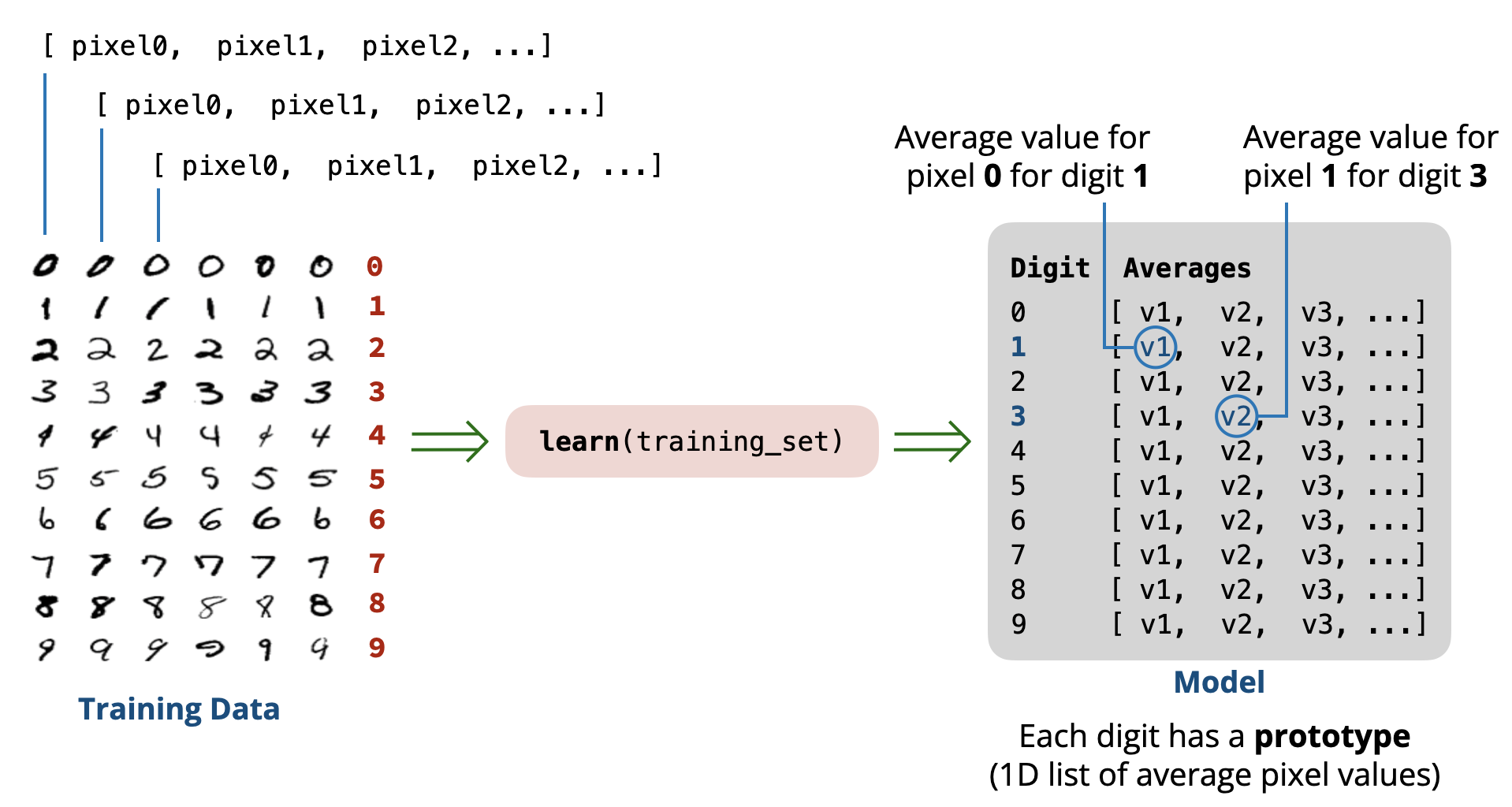
Learning Phase: We will use the training set to learn the average pixel value at each pixel position. This gives us a prototype image for each digit (a 1D list of \(28\times28=784\) average pixel values).

Prediction Phase: When asked to predict the digit in a new image, we will compute the difference (distance) between the pixel values of the image and each prototype image for the digits \((0-9)\). The predicted digit will be the one whose prototype image is closest to the new image (minimum distance).

Using this approach, if a digit tends to have more dark pixels in certain locations, the prototype image will reflect that, and the classifier can use this information to make better predictions.

Learning Phase

Let’s start by implementing a function that goes through all the images in the training set for a single digit and computes the average pixel value at each pixel position.

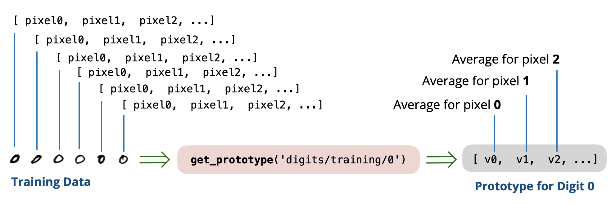
def get_prototype(folder):
    sum_pixels = [0] * (28 * 28)
    count = 0

    # Loop over each file in the folder
    for filename in os.listdir(folder):
        fullname = folder + '/' + filename
        pixels = read_as_1D(fullname)

        # update the sum for every pixel position
        for i in range(len(pixels)):
            sum_pixels[i] += pixels[i]

        count += 1

    # compute average at each pixel position
    avg_pixels = [0] * (28 * 28)
    for i in range(len(sum_pixels)):
        avg_pixels[i] = sum_pixels[i] / count

    return avg_pixels

Using this function, we can compute the prototype images for all digits \((0-9)\) as follows:

def get_prototypes(training_folder):
    prototypes = []

    # Loop over each digit (0-9)
    for digit in '0123456789':
        folder = training_folder + '/' + digit
        print('Creating Prototype for digit:', digit)

        prototype = get_prototype(folder)
        prototypes.append(prototype)
    
    return prototypes

The result is a list of \(10\) prototype images, each represented as a 1D list of \(784\) average pixel values. In other words, the result is a 2D list of size \(10\) rows \(\times\) \(784\) columns.

[
  [avg0, avg1, avg2, ..., avg783], # prototype for digit 0
  [avg0, avg1, avg2, ..., avg783], # prototype for digit 1
  [avg0, avg1, avg2, ..., avg783], # prototype for digit 2
   ..., 
  [avg0, avg1, avg2, ..., avg783]  # prototype for digit 9
]

The following is a visualization of the prototype images for all digits:

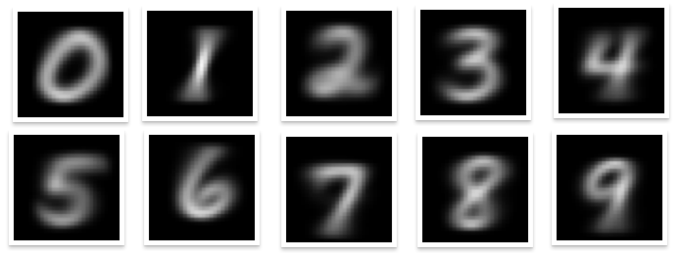
The blurry parts in the images represent where the digit is likely to have white pixels. This is exactly what we want!

Note. We will not work with the prototype images directly. Instead, we will use the 1D lists of average pixel values that represent these images. If you are curious, you can inspect the following code that was used to generate the above visualization.

Optional Code

def create_average_image(digit_folder, output_file):
    sum_pixels = [0] * (28 * 28)
    count = 0
    
    for file in os.listdir(digit_folder):
        pixels = read_as_1D(digit_folder + '/' + file)
        
        for i in range(len(pixels)):
            sum_pixels[i] += pixels[i]
        
        count += 1
    
    avg_pixels = []
    for i in range(len(sum_pixels)):
        avg_pixels.append(int(sum_pixels[i] / count))
    
    image = Image.new('L', (28, 28))
    image.putdata(avg_pixels)
    image.save(output_file)

for digit in '0123456789':
    print('Creating average image for digit', digit)
    create_average_image('digits/training/' + digit, 
                         f'average_{digit}.png')

Distance Function

To compare a new image to the prototype images, we need a function that computes the distance between two images \(p\) and \(q\) (represented as 1D lists of pixel values). A common choice is the Euclidean distance:

\[d(p, q) = \sqrt{(p_0 - q_0)^2 + (p_1 - q_1)^2 + ... + (p_{783} - q_{783})^2}\]

import math
def distance(p, q):
    total = 0
    for i in range(len(p)):
        total += (p[i] - q[i]) ** 2
    return math.sqrt(total)

Testing Phase

We are now ready to check the performance of our improved classifier on the test set. The predict function will compare the new image to each prototype and return the digit of the closest prototype.

def predict(image, prototypes):
    pixels = read_as_1D(image)

    min_dist = None
    result = None

    # Compare to each prototype
    for digit in range(10):
        dist = distance(pixels, prototypes[digit])
        if min_dist == None or dist < min_dist:
            min_dist = dist
            result = str(digit)

    return result

prototypes = get_prototypes('digits/training')
evaluate('digits/testing', prototypes)

The above code requires a small modification to the evaluate function to accept the prototypes as an argument and use the new predict function that takes the prototypes as argument.

def evaluate(test_folder, prototypes): # <-- modified
    correct = 0     
    count = 0       
    
    for digit in '0123456789':
        folder = test_folder + '/' + digit

        for file in os.listdir(folder):
            fullname = folder + '/' + file
            print('Evaluating image:', fullname)

            prediction = predict(fullname, prototypes) # <-- modified
            if prediction == digit:
                correct += 1
            count += 1
            
    print('Accuracy:', correct / count * 100, '%')

Running the evaluation gives us an accuracy of about 82.03%. This is a huge improvement over our previous attempt (\(22\%\) accuracy)! 🎉🎉

However, there is still room for improvement.

DEFINITION
The approach we just implemented is called a Nearest Prototype Classifier. In such a classifier, each class (digit in our case) is represented by a prototype representing the main properties of that class, and new instances are classified based on their proximity to these prototypes.

Are All Pixels Positions Equally Important?

In our current model, we treat all pixel positions equally when computing the distance between images. For example, a difference in pixel values in the center of the image affects the computed distance just as much as a difference in pixel values in the corners of the image.

However, intuitively, some pixel positions are more important than others, especially for differentiating between certain digits. This important observation will be the basis for our next attempt to improve the classifier’s performance.

Next Steps

In the next lesson, we will explore a method that allows us to assign different importance (weights) to different pixel positions when making predictions.