Machine Learning (Part 1)
Table of contents
- Overview
- Machine Learning
- Problem Overview
- The Dataset
- Before We Start
- Attempt # 1
- A Closer Look at Our Approach
Overview
This is the first of 3 parts on Machine Learning (ML). The goal of these lessons is to give you an introduction to ML concepts through a hands-on application. In this part, we will introduce the ML application along with some naive solutions. The goal is to illustrate key ML concepts and pave the way for more advanced solutions in the next parts.
Machine Learning
Machine learning is currently the hottest subfield of Artificial Intelligence (AI). Anyone working in AI today is likely to be working on machine learning.
At a high level, machine learning is about building computer systems that can learn from data to make predictions or decisions.
DEFINITION
Learning is the process of improving the performance on a task based on experience.
A player is said to be learning how to play chess if their performance in playing chess improves over time with practice (experience). A child is said to be learning to recognize animals if their ability to identify different animals improves as they are exposed to more animals.
In the context of machine learning, the experience usually comes in the form of a dataset of examples that the system can learn from. For instance, a system that recognizes human faces can learn from a dataset of images of human faces, and a system that predicts stock prices can learn from a dataset of historical stock prices.
Problem Overview
We are given a dataset of images of handwritten digits \((0-9)\) and are asked to use it to build a system that can take an image of a handwritten digit \((0-9)\) and predict which digit it is.
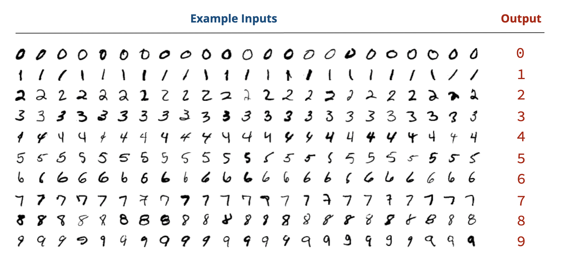
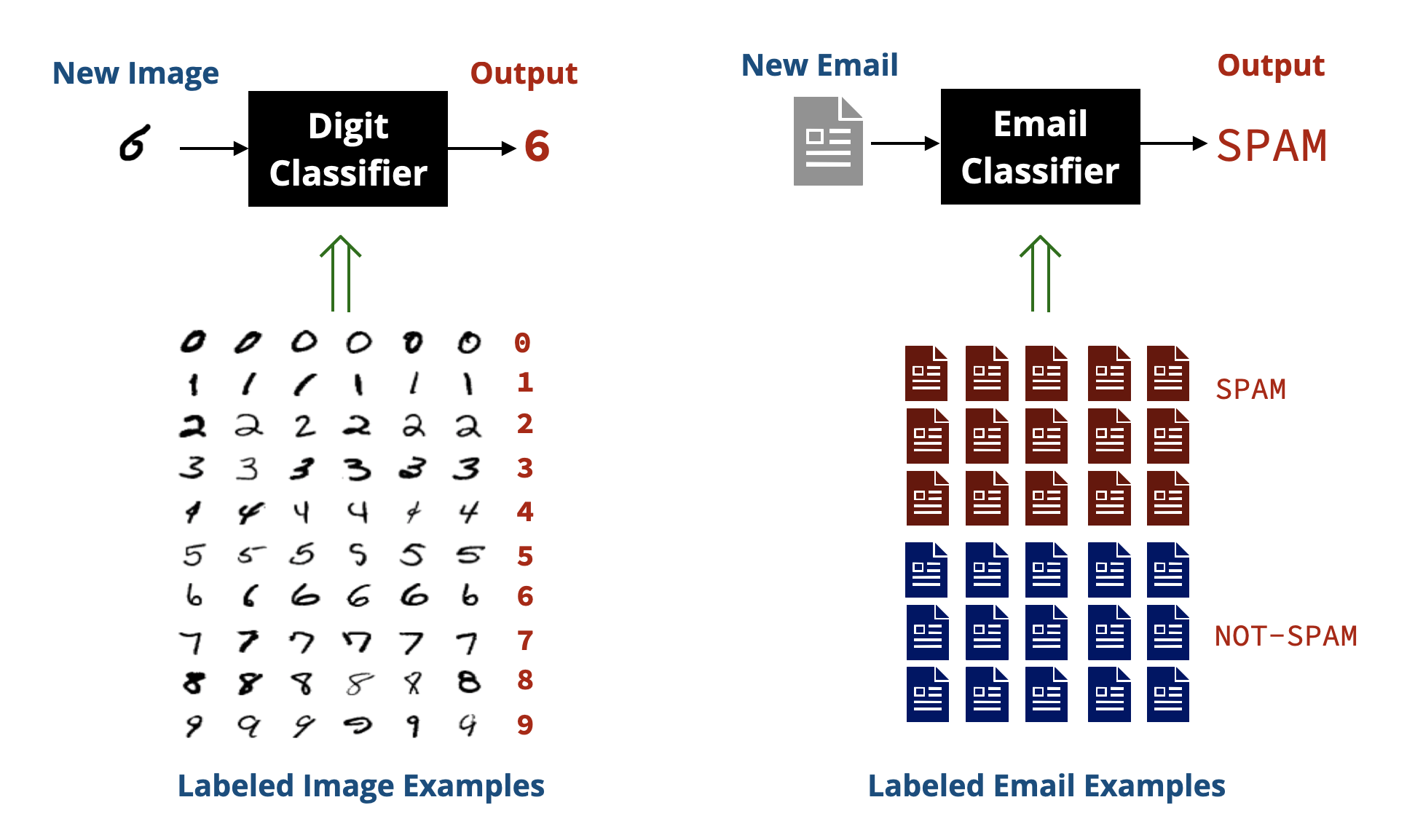
This problem is a classical example of what is called classification in ML, where the goal is to assign an input (e.g., an image) to one of several categories (e.g., the digits \(0-9\)). Other examples of classification problems include classifying emails as spam or not spam, classifying product reviews as positive or negative, and classifying medical images as showing signs of a disease or not.
In a classification problem, we have a dataset of examples that are already classified (labeled), which the system can learn from.
The Dataset
We will be using the MNIST dataset, which is a well-known dataset of handwritten digits. The data is split into:
Training set: \(60,000\) images of handwritten digits along with their labels (the digit they represent). This is the data that our system is allowed to learn from.
Test set: \(10,000\) images of handwritten digits along with their labels. This is the data that we will use to evaluate how well our system performs on unseen data.
Each image in the dataset is a \(28 \times 28\) pixel grayscale image. The background is black (pixel value \(0\)), and the digit is drawn in white (pixel value \(255\)) with varying shades of gray in between.
The images are organized in folders, where each folder corresponds to a digit \((0-9)\). The following screen recording shows the structure of the dataset:
Before We Start
Before we start building our solution, let’s define the main functions we will be using throughout this lesson:
1. read_as_1D(filename)
This function takes the name of an image file as an argument and returns its pixel values as a 1D list (i.e., a list of \(28 \times 28 = 784\) elements). Each pixel value is an integer between \(0\) and \(255\).
from PIL import Image

def read_as_1D(filename):
    # Open the image in grayscale
    # (using convert('L') makes each pixel a single value 0-255)
    image = Image.open(filename).convert('L')

    # Get pixel values as a 1D list
    return list(image.getdata())
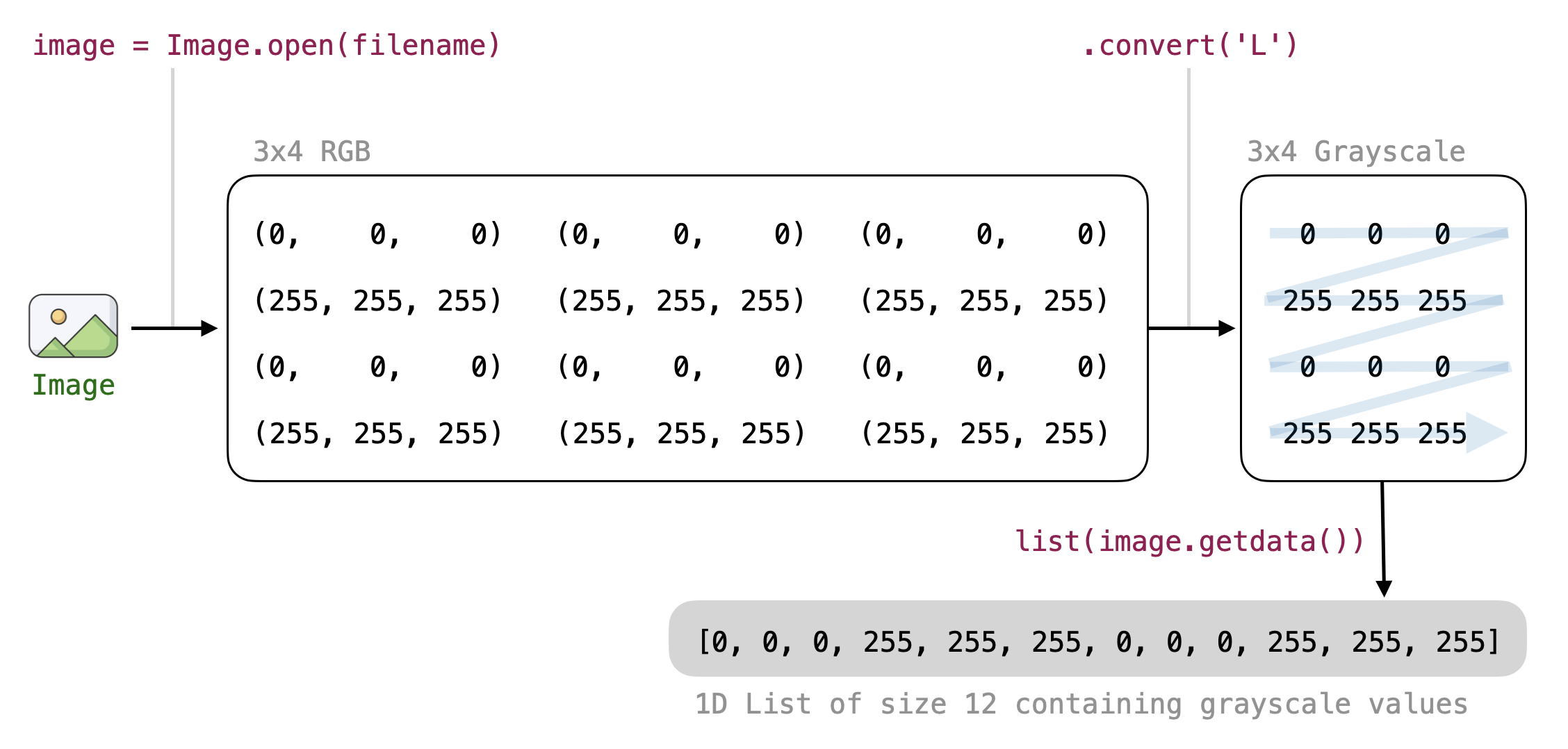
In many cases, we want to perform operations on all the pixel values of an image regardless of their 2D position (e.g., computing the average pixel value). Having a list of pixel values makes writing the code for such operations easier.
2. predict(image)
This function takes the name of an image file as input and returns the predicted label (digit) for that image. Most of our work will be focused on implementing this function.
3. evaluate(test_folder)
This function takes the name of the folder containing test data and produces an accuracy score indicating how well our predict function performs on the given test data.
Since the test data is organized into subfolders (one for each digit), the function will need to loop over each subfolder and each image file in that subfolder, send the image to the predict function, and compare the predicted label with the actual label (the name of the subfolder).
import os

def evaluate(test_folder):
    correct = 0     # Number of correct predictions
    count = 0       # Total number of predictions

    # Loop over each folder (0-9)
    for digit in '0123456789':
        folder = test_folder + '/' + digit

        # Loop over each file in the folder
        for file in os.listdir(folder):
            fullname = folder + '/' + file
            print('Evaluating image:', fullname)

            if predict(fullname) == digit:
                correct += 1
            count += 1

    print('Accuracy:', correct / count * 100, '%')

# Dummy predict function: Always predicts '0'
# We will improve this function later
def predict(image):
    return '0'
Assuming the function is called as evaluate('digits/testing'), the outer loop goes over the folders named:
digits/testing/0
digits/testing/1
digits/testing/2
...
digits/testing/9
For each folder, the inner loop goes over each image file in that folder and sends it to the predict function to get a prediction. If the prediction matches the folder name, we increment the correct counter.
A PYTHON NOTE
The
os.listdir(folder)function returns a list of all files and directories in the specified folder. We use it here to loop over all image files in each digit folder.
Here is how the files are visited by the above code:
folder: digits/testing/0
            fullname: digits/testing/0/1.png
            fullname: digits/testing/0/2.png
            fullname: digits/testing/0/3.png
            ...
folder: digits/testing/1
            fullname: digits/testing/1/1.png
            fullname: digits/testing/1/2.png
            fullname: digits/testing/1/3.png
            ...
...
folder: digits/testing/9
            fullname: digits/testing/9/1.png
            fullname: digits/testing/9/2.png
            fullname: digits/testing/9/3.png
            ...
Baseline Performance
If we run the above code with the dummy predict function that always returns 0, we will get an accuracy of around 10% since only the images in the 0 folder will be predicted correctly (out of \(10,000\) images, only around \(1,000\) are 0s).
Attempt # 1
A Simplified Version
Before we attempt the full problem, let’s first attempt a simplified version of it. We will assume that our test set only contains images of 0s and 1s and our goal is to build a predict function that can distinguish between these two digits only.
We can easily modify our evaluate function to only consider these two digits by changing the outer loop to be:
for digit in '01':
Instead of:
for digit in '0123456789':
Running the code again with the dummy predict function that always returns 0 will now give us an accuracy of around \(46\%\) since half of the images in the test set are 0s and the other half are 1s.
A Simple Approach
How can we distinguish between 0s and 1s? One simple idea is to look at how black or white the image is. Intuitively, 0s might have more white pixels than 1s since 0s are a closed loop, while 1s are a straight line.
Let’s begin by writing a function that computes the average pixel value of an image.
def average(pixels):
    return sum(pixels) / len(pixels)

# Example usage:
pixels = read_as_1D('digits/training/1/1.png')
print('Average:', average(pixels))
We can apply the above function to all the 0 images in the training set to compute the average pixel value for the digit 0, and do the same with all the 1 images to get the average for 1.
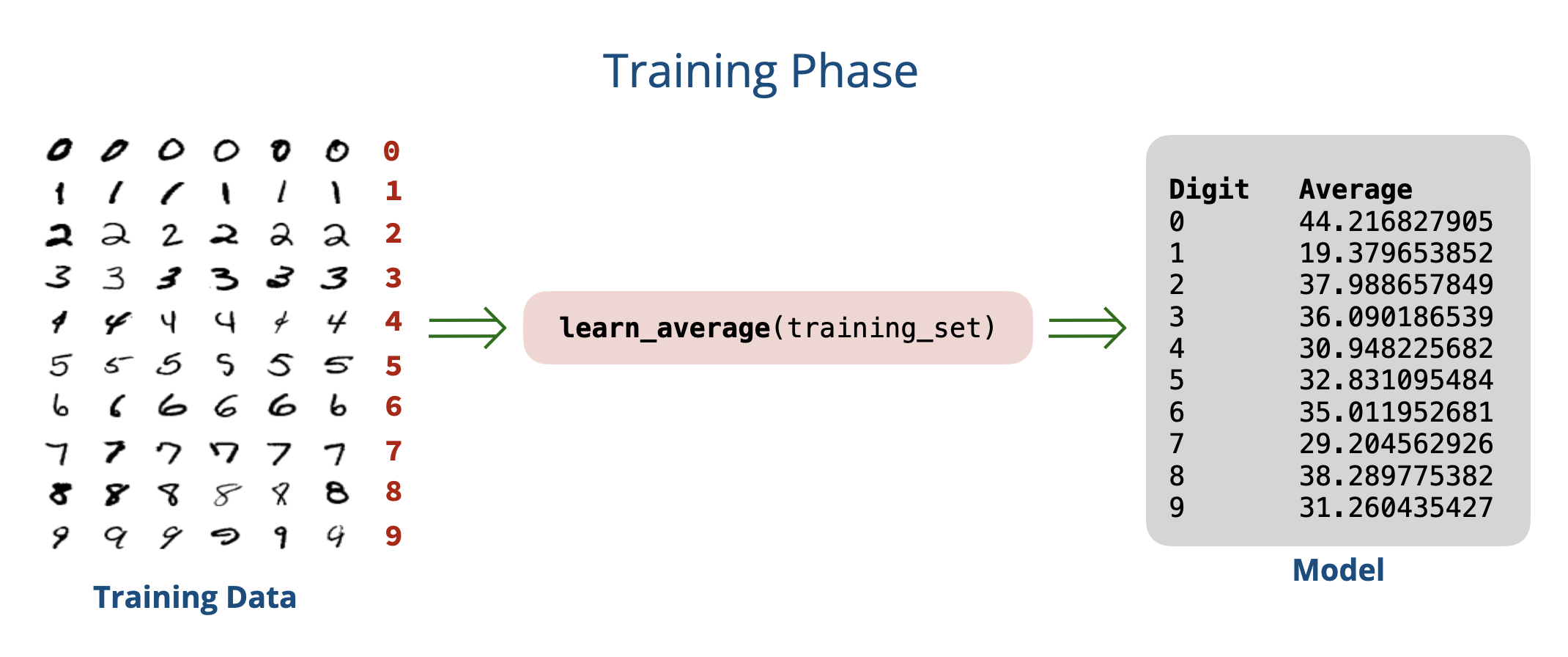
In other words, we want to learn the average pixel value for each digit from the training data.
def learn_average(digit_folder):
    total = 0
    count = 0

    for file in os.listdir(digit_folder):
        pixels = read_as_1D(digit_folder + '/' + file)
        total += average(pixels)
        count += 1

    return total / count

print('Learning average for 0 ...')
avg0 = learn_average('digits/training/0')

print('Learning average for 1 ...')
avg1 = learn_average('digits/training/1')

print('Average for 0:', avg0)
print('Average for 1:', avg1)
Running the above code gives us the following average pixel values:
Average for 0: 44.21682790539817
Average for 1: 19.379653852789957
This confirms our intuition that 0s tend to have more white pixels (higher average pixel value) than 1s.
Let’s use this information to build our predict function:
# Predict if the image is a 0 or a 1
def predict(image):
    AVERAGES = [44.21682790539817,    # learned average for '0'
                19.379653852789957]   # learned average for '1'

    pixels = read_as_1D(image)
    avg = average(pixels)

    # Predict '0' if avg is closer to the average for '0'
    # Otherwise, predict '1'
    if abs(avg - AVERAGES[0]) < abs(avg - AVERAGES[1]):
        return '0'
    else:
        return '1'
Let’s evaluate our predict function on the simplified test set containing only 0s and 1s:
>>> evaluate('digits/testing')
Accuracy:  92.72%
This is huge! We managed to achieve over \(90\%\) accuracy simply by comparing average pixel values! 🎉🎉
Generalizing to All Digits
Let’s apply the same approach for the full problem (digits \(0-9\)) by learning the average pixel value for each digit:
print('Digit\t Average')
for digit in '0123456789':
    folder = 'digits/training/' + digit
    avg = learn_average(folder)
    print(digit, '\t', avg)
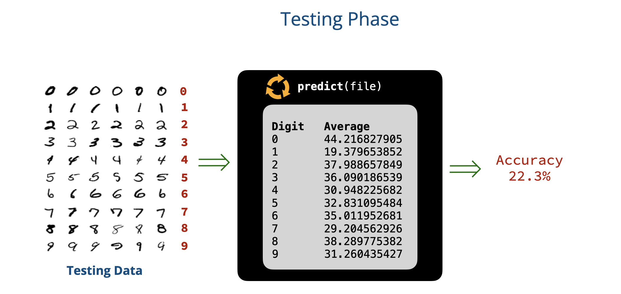
Running the above code gives us the following average pixel values for all digits:
Digit   Average
0       44.21682790539817
1       19.379653852789957
2       37.988657849846874
3       36.09018653946659
4       30.948225682775707
5       32.83109548467975
6       35.011952681545765
7       29.204562926527398
8       38.2897753828927
9       31.260435427322733
Let’s update our predict function to handle all digits:
def predict(image):
    AVERAGES = [
        44.21682790539817,
        19.379653852789957,
        37.988657849846874,
        36.09018653946659,
        30.948225682775707,
        32.83109548467975,
        35.011952681545765,
        29.204562926527398,
        38.2897753828927,
        31.260435427322733
    ]

    pixels = read_as_1D(image)
    avg = average(pixels)

    # Find the closest digit based on average pixel value
    min_diff = None
    closest_digit = None
    for i in range(10):
        diff = abs(avg - AVERAGES[i])
        if min_diff is None or diff < min_diff:
            min_diff = diff
            closest_digit = i

    return str(closest_digit)
We can now evaluate our predict function again to see how well it performs on the full dataset.
What do we get?
>>> evaluate('digits/testing')
Accuracy: 22.3 %
This is catastrophically bad! 🤦♂️🤦♂️
We should have been less optimistic about this simple approach. But why?
While it worked well for distinguishing between 0s and 1s, the average pixel value fails to capture the complexity of the other digits. For example, digits like 2, 3, and 5 have similar average pixel values.
One problem in our approach is that we completely ignore where pixels are. Two images can have the same average pixel value but look completely different. We need to capture and use more information about the images to improve our predictions.
A Closer Look at Our Approach
Architecture
Our approach in Attempt # 1 can be split into two phases:
- Training phase: In this phase, we learned from the training data by computing the average pixel value for each digit \((0-9)\). The result of this phase is a set of learned averages that we used for prediction. We will refer to these learned averages as our model.
- Testing phase: In this phase, we used our learned model to make predictions on new images. To check how well our model performs, we checked the accuracy of our predictions on the images in the test set and computed an accuracy score.
Shortcomings of Our Approach
The problem with our approach is that the model we learned is too simplistic:
- First, it only captures a single feature of the image: the average pixel value.
- Second, it bases its predictions on a very simple rule: choosing the digit whose average pixel value is closest to that of the input image.
To improve our model, we need to use more and better features of the image (instead of the single value we are currently using), and use a more sophisticated method to combine these features to make predictions.
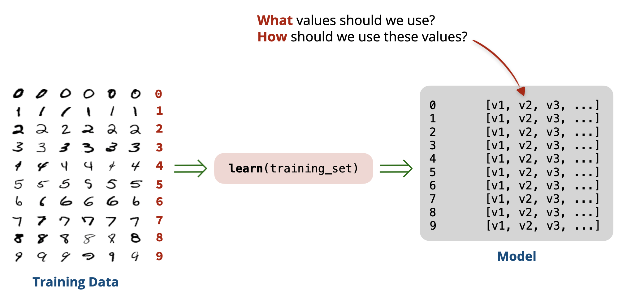
What features should we consider? And how should we combine them? This is the essence of machine learning, and we will explore these questions in the next parts of this lesson.