Algorithms and Efficiency
Table of contents
- Introduction
- Timing Code Execution
- Appending and Prepending to Lists
- Predicting Running Time
- Fixing The Problem
- Removing All Occurrences of An Element
- Counting Distinct Elements
- Sum of Squares
- Summary
Introduction
When writing short pieceis of code that process small amounts of data (like the ones we have been writing so far), efficiency is not a big concern. In fact, it is often in such cases better to write code that is easy to read and understand, even if it is not the most efficient. However, in real-world applications, we often need to process large amounts of data, or perform operations that need to be done very quickly. In such cases, efficiency becomes a critical factor.
For example, you would not be happy if:
- Google took several minutes to return results for a query.
- Instagram took several minutes to load your feed.
- Your favorite video game lagged and froze every few seconds.
In this lesson, we will discuss algorithm efficiency, which is one of the most important concepts in computer science. A large part of computer science is dedicated to designing efficient algorithms that can process large amounts of data quickly, and to analyzing the memory and time requirements of different algorithms.
Timing Code Execution
One way to measure the efficiency of an algorithm is to measure the time it takes to execute. In Python, we can use the time module to measure the execution time of a piece of code. Here is an example:
import time

start = time.time()

# Code to be timed

end = time.time()
total_time = end - start
print("Execution time:", total_time, "seconds")
The idea is to record the time before and after the code execution, and then calculate the difference. This gives us the total time taken to execute the code.
Appending and Prepending to Lists
Let’s compare the running time of the following two pieces of code:
numbers = []
for _ in range(N):
    numbers += [randint(1, 100)]
and
numbers = []
for _ in range(N):
    numbers = [randint(1, 100)] + numbers
Both pieces of code generate a list of random numbers. The first code appends numbers to the end of the list, while the second code prepends numbers at the beginning of the list. The following code measures the running time of both methods:
import time
from random import randint

N = int(input("How many numbers? "))

# Appending
start = time.time()
numbers = []
for _ in range(N):
    numbers += [randint(1, 100)]
end = time.time()
print("Appending:", end - start, "seconds")

# Prepending
start = time.time()
numbers = []
for _ in range(N):
    numbers = [randint(1, 100)] + numbers
end = time.time()
print("Prepending:", end - start, "seconds")
These two programs look very similar. If we run them with N=10000, we get:
Appending : 0.005068063735961914 seconds
Prepending: 0.08214592933654785 seconds
Both methods finish in lightning speed, but the second method seems a bit slower. Let’s double \(N\) to \(20000\) and see what happens:
Appending : 0.009379148483276367 seconds
Prepending: 0.3352389335632324 seconds
The second method is clearly slower, but still manageable. Let’s try with \(N=40000\), \(N=80000\), and \(N=160000\). Here is a summary of the results we get:
Appending:
Size     Time (seconds)
---------------------------
10000    0.005068063735961
20000    0.009379148483276
40000    0.018888950347900
80000    0.037770986557006
160000   0.067885875701904
Prepending:
Size     Time (seconds)
---------------------------
10000    0.082145929336547
20000    0.335238933563232
40000    1.266126155853271
80000    4.950298070907593
160000   19.97136688232422
Now, the second method is clearly taking significantly more amount of time. Thinking of it, \(80,000\) and \(160,000\) are not that large. In fact, many applications today deal with millions or even billions of data points. Performing so slowly on such small inputs is definitely not acceptable.
So, what is going on here? Why is the second method so much slower than the first? The answer lies in the way lists are implemented in Python. When you create a list, Python allocates a contiguous block of memory to store the list elements. This block is fixed in size. Therefore:
- Python reserves extra space, so that appending to the end of the list (using
appendor+=) can be done quickly in the next available empty slot in the list.
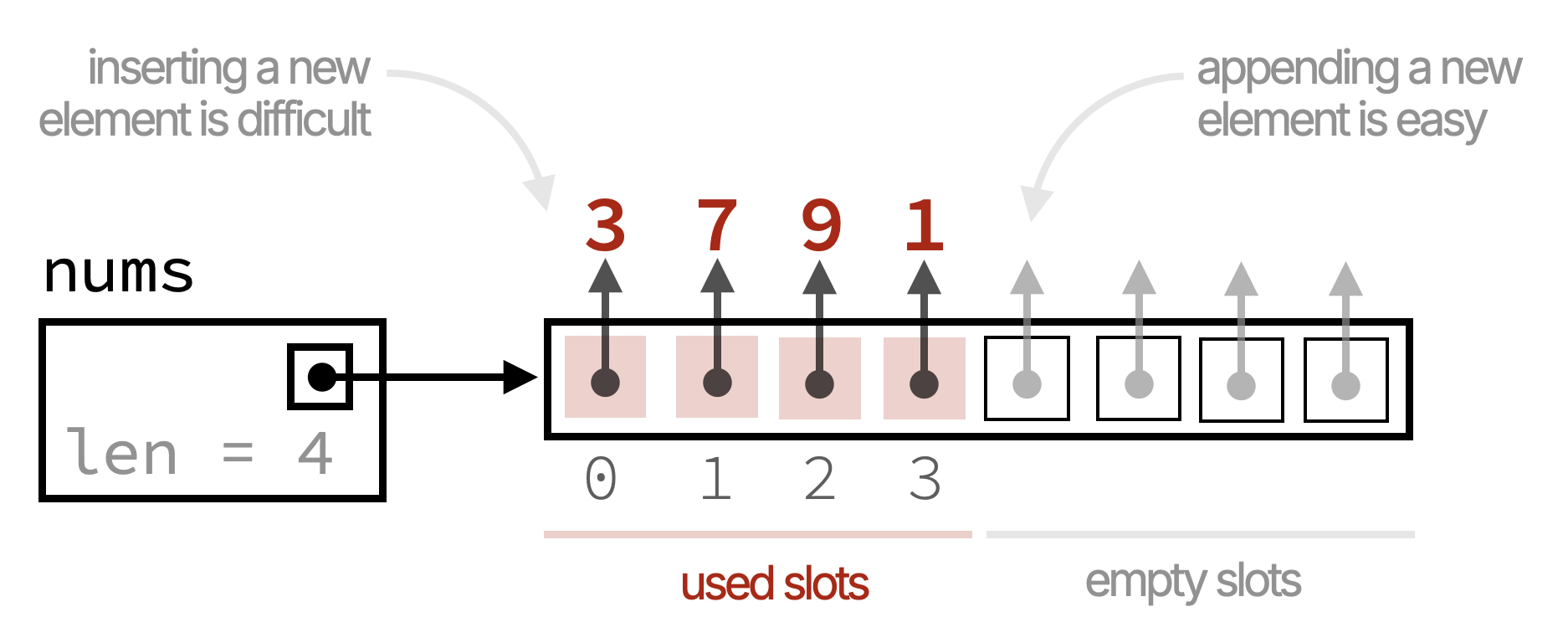
- Adding to the beginning of the list is not easy, because there are no empty slots! The operation
numbers = [randint(1, 100)] + numberscreates a new list and copies all the elements from the original list to the new list with the new element added at the beginning.
This means that for each insertion at the beginning, Python has to copy all the existing elements to a new location in memory, which takes a lot of time if there are many elements in the list.
Predicting Running Time
How much time will each method take if we increase \(N\) to one billion?
Let’s take a closer look at the running times we observed for the two methods:
Appending:
| Size     | Time      | Ratio |
|----------|-----------|-------|
| 10,000   | 0.0051s   |  -    |
| 20,000   | 0.0094s   | ≈ 1.8 |
| 40,000   | 0.0189s   | ≈ 2.0 |
| 80,000   | 0.0378s   | ≈ 2.0 |
| 160,000  | 0.0679s   | ≈ 1.8 |
We can see that the running time roughly doubles when we double the size of the list. This is good!
Let’s now look at the prepending operation:
Prepending:
| Size     | Time     | Ratio |
|----------|----------|-------|
| 10,000   | 0.0821s  |  -    |
| 20,000   | 0.3352s  | ≈ 4   |
| 40,000   | 1.2661s  | ≈ 3.8 |
| 80,000   | 4.9503s  | ≈ 3.9 |
| 160,000  | 19.971s  | ≈ 4.0 |
We can see that the running time roughly quadruples (is multipled by ≈ 4) when we double the size of the list. This is bad!
From these observations, we can make a rough prediction of the running time for larger sizes. For example, if we want to estimate the time for \(N=320,000\):
- Appending: We can expect the time to be around \(0.0679s \times 2 ≈ 0.1372\) seconds.
- Prepending: We can expect the time to be around \(19.9714s \times 4 ≈ 79.8856s ≈ 1.33\) minutes.
We definitely do not want to run the program for one billion numbers. If takes around a minute for \(160,000\) numbers, who knows how long it will take for one billion!
Instead, we will download and use time_plot.py, which allows making time predictions based on previous running times. Using the tool, we get the following predictions for \(N=1,000,000,000\):
- Appending: \(4.67\) minutes.
- Prepending: \(19.41\) years.
You have seen it right! The prepend operation will take almost two decades to finish! This is clearly unacceptable.
Fixing The Problem
Another way to achieve the same effect of prepending to a list is to create a new list of size \(N\), and then fill it from the end to the beginning (backwards). Here is the code:
numbers = [0] * N
for i in range(N):
    numbers[N - 1 - i] = randint(1, 100)
Let’s time this code for different values of \(N\):
import time
from random import randint

for N in [10000, 20000, 40000, 80000, 160000]:
    start = time.time()

    numbers = [0] * N
    for i in range(N):
        numbers[N - 1 - i] = randint(1, 100)

    end = time.time()
    print(N, '\t', end - start, 'seconds')
Running this code gives the following results:
N        Time (seconds)
----------------------------
10000    0.00523400306701660
20000    0.00986909866333007
40000    0.01919674873352050
80000    0.03620004653930664
160000   0.06852579116821289
Now, the running times are comparable to the append operation. This is because we are no longer creating a new list and copying elements for each insertion. Instead, we are simply filling in the pre-allocated list, which is much more efficient.
Removing All Occurrences of An Element
Let’s see another example that illustrates the importance of algorithm efficiency.
Suppose we want to remove all occurrences of a value x from a list named nums. Here is a simple implementation:
while x in nums:
    nums.remove(x)
How efficient is this code? Let’s put it in a loop that doubles the size of the list each time, and see how long it takes to remove all occurrences of x:
import time
from random import randint

for N in [10000, 20000, 40000, 80000, 160000]:
    # Generate a list with random numbers between 1 and 10
    numbers = []
    for _ in range(N):
        numbers.append(randint(1, 10))
    x = randint(1, 10)

    # Remove all occurrences of x
    start = time.time()
    while x in numbers:
        numbers.remove(x)
    end = time.time()

    print(N, '\t', end - start, 'seconds')
Running this code and computing the ratios gives the following results:
|  N     | Time (seconds) | Ratio  |
|--------|----------------|--------|
| 10000  | 0.10663509368  |  -     |
| 20000  | 0.46504402160  | ≈ 4.36 |
| 40000  | 1.58694624900  | ≈ 3.41 |
| 80000  | 6.11097311973  | ≈ 3.85 |
| 160000 | 25.1159579753  | ≈ 4.11 |
These results exhibit the same dreaded quadrupling behavior we saw earlier! Moving from \(80,000\) to \(160,000\) takes us from about \(6.1\) seconds to about \(25.1\) seconds. This is clearly inefficient and is expected to take years for one billion elements.
Why is this code so inefficient? The reason is twofold:
- In each iteration of the
whileloop, we use theinoperator to check ifxis in the list. This requires scanning the entire list. - If
xis found, we use theremovemethod to remove the first occurrence ofx. This also requires scanning the list to findx, and then shifting all subsequent elements to fill the gap caused by removingx.
To fix this problem, we can use a similar approach to the one we used for prepending. We can create a new list and copy only the elements that are not equal to x. Here is the code:
# copy all elements that are not x to a new list
result = []
for num in numbers:
    if num != x:
        result.append(num)

# assign the new list back to numbers
numbers = result
Here is the complete timing code with this modified method:
import time
from random import randint

for N in [10000, 20000, 40000, 80000, 160000]:
    # Generate a list with random numbers between 1 and 10
    numbers = []
    for _ in range(N):
        numbers.append(randint(1, 10))
    x = randint(1, 10)

    # Remove all occurrences of x
    start = time.time()
    result = []
    for num in numbers:
        if num != x:
            result.append(num)
    numbers = result
    end = time.time()

    print(N, '\t', end - start, 'seconds')
Running this code gives the following results:
|  N     |  Time (seconds) | Ratio  |
|--------|-----------------|--------|
| 10000  |  0.00146579742  | -      |
| 20000  |  0.00280594825  | ≈ 1.91 |
| 40000  |  0.00660872459  | ≈ 2.36 |
| 80000  |  0.01396870613  | ≈ 2.11 |
| 160000 |  0.02176904678  | ≈ 1.56 |
Now, the running times are much more reasonable and they roughly double when we double the size of the list.
Counting Distinct Elements
Suppose we want to count the number of distinct elements in a list named numbers. Here is a simple implementation:
def count_distinct(numbers):
    distinct = []
    for num in numbers:
        if num not in distinct:
            distinct.append(num)
    return len(distinct)
Based on our previous discussion, we should expect this code to be inefficient, as each iteration of the for loop uses the in operator to scan the distinct list searching for num. Indeed, running the following code gives us the same dreaded quadrupling behavior!
for N in [10000, 20000, 40000, 80000, 160000]:
    # Generate a list with random numbers between 1 and 10
    numbers = []
    for _ in range(N):
        numbers.append(randint(1, N))

    start = time.time()
    count_distinct(numbers)
    end = time.time()
    print(N, '\t', end - start, 'seconds')
|  N     | Time (seconds) | Ratio  |
|--------|----------------|--------|
| 10000  | 0.335536956787 | -      |
| 20000  | 1.332063913345 | ≈ 4    |
| 40000  | 4.868139982223 | ≈ 3.65 |
| 80000  | 19.12762379646 | ≈ 3.93 |
| 160000 | 87.21093606948 | ≈ 4.56 |
Can you think of a more efficient way to count the number of distinct elements in a list? Here is an observation that can help:
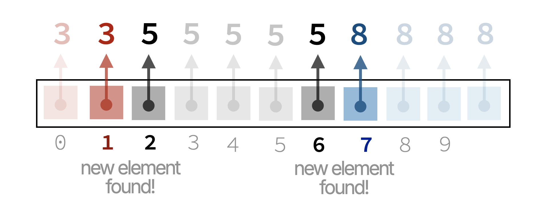
If we sort the list first, then all occurrences of the same element will be adjacent to each other. For example, the list \([3,\ 5,\ 8,\ 5,\ 3,\ 5,\ 8,\ 5,\ 5,\ 8,\ 8]\) becomes \([3, 3,\ 5, 5, 5, 5, 5,\ 8, 8, 8, 8]\) after sorting.
Since equal elements are adjacent, we can simply iterate through the sorted list and count how many times we encounter a new element.
Here is the modified code:
def count_distinct(numbers):
    if not numbers:
        return 0

    numbers.sort()
    count = 1
    for i in range(1, len(numbers)):
        if numbers[i] != numbers[i - 1]:
            count += 1
    return count
Running the same timing code with this modified function gives us the following results:
|  N     | Time (seconds) | Ratio  |
|--------|----------------|--------|
| 10000  | 0.002504348754 | -      |
| 20000  | 0.005484104156 | ≈ 2.19 |
| 40000  | 0.010379076004 | ≈ 1.89 |
| 80000  | 0.020861864090 | ≈ 2.01 |
| 160000 | 0.038151979446 | ≈ 1.83 |
This is lightning fast compared to the previous implementation! The quaderupling behavior is gone, and the running time roughly doubles when we double the size of the list.
Sum of Squares
Given a number \(c\), we want to check if there exist two integers \(a\) and \(b\) such that \(a^2 + b^2 = c\).
The most straightforward way to solve this problem is to use two nested loops to iterate through all possible values of \(a\) and \(b\), and check if the equation holds. Here is the code:
def check(c):
    for a in range(1, c):
        for b in range(1, c):
            if a * a + b * b == c:
                return True
    return False
If \(c = 4\), the code above checks the following pairs \((a, b)\):
\[1^2 + 1^2\] \[1^2 + 2^2\] \[1^2 + 3^2\]
\[2^2 + 1^2\] \[2^2 + 2^2\] \[2^2 + 3^2\]
\[3^2 + 1^2\] \[3^2 + 2^2\] \[3^2 + 3^2\]
Let’s time this code for different values of \(c\):
import time

for c in [10000, 20000, 40000, 80000, 160000]:
    start = time.time()
    check(c)
    end = time.time()
    print(c, '\t', end - start, 'seconds')
We should expect the running time to be different based on whether \(c = a^2 + b^2\) for some pair \((a, b)\) or not. If such a pair is found early, the function will return quickly. However, if no such pair exists, the function will have to check all possible pairs.
|  c     | Time (seconds) | Ratio   |
|--------|----------------|---------|
| 10000  | 0.022106170654 | -       |
| 20000  | 0.028832197189 | ≈ 1.30  |
| 40000  | 0.168849945068 | ≈ 5.86  |
| 80000  | 0.268959999084 | ≈ 1.59  |
| 160000 | 1.670704126358 | ≈ 6.21  |
Indeed, we see that the running time varies significantly based on the input value of \(c\). Let’s redo the experiment, this time using values for \(c\) that are almost doubles of each other, but all of which do not have such a pair \((a, b)\):
|  c     | Time (seconds) | Ratio   |
|--------|----------------|---------|
| 999    | 0.076351165771 | -       |
| 1999   | 0.270452022552 | ≈ 3.54  |
| 3999   | 1.098377943039 | ≈ 4.06  |
| 8001   | 4.693326950073 | ≈ 4.27  |
| 15999  | 19.48631334304 | ≈ 4.15  |
The dreaded quadrupling behavior is back again! This is because the if \(c = 999\), our code has to check \(998 \times 998 = 996004\) pairs of \((a, b)\). However, is this really necessary?
Let’s improve our algorithm. The first thing to notice is that we are checking pairs \((a, b)\) and \((b, a)\) separately, even though they yield the same result. For example, why check \(1^2 + 2^2\) and \(2^2 + 1^2\)? They have the same sum, so checking only one is enough.
We can modify our code to only check pairs where \(b \geq a\):
def check(c):
    for a in range(1, c):
        for b in range(a, c):
            if a * a + b * b == c:
                return True
    return False
If \(c = 4\), the modified code checks the following pairs \((a, b)\):
\[1^2 + 1^2\] \[1^2 + 2^2\] \[1^2 + 3^2\]
\[\color{red}\cancel{2^2 + 1^2}\] \[2^2 + 2^2\] \[2^2 + 3^2\]
\[\color{red}\cancel{3^2 + 1^2}\] \[\color{red}\cancel{3^2 + 2^2}\] \[3^2 + 3^2\]
Clearly, this will get rid of many redundant checks. Let’s time this modified code to see how much of an improvement we get:
|  c     | Time (seconds) | Ratio   |
|--------|----------------|---------|
| 999    | 0.040757894515 | -       |
| 2001   | 0.141206979751 | ≈ 3.47  |
| 3999   | 0.596912860870 | ≈ 4.23  |
| 8001   | 2.227569818497 | ≈ 3.73  |
| 15999  | 8.727083921432 | ≈ 3.92  |
While the running times are cut in half compared to the previous implementation, we still see the dreaded quadrupling behavior. Can we do better?
Yes! Note the following:
No number above \(\sqrt{c}\) can be part of a valid pair \((a, b)\).
If \(a > \sqrt{c}\), then \(a^2 + b^2 > c\). Therefore, we can modify our code to only check values of \(a\) and \(b\) up to \(\sqrt{c}\):
def check(c):
    limit = int(c ** 0.5) + 1
    for a in range(1, limit):
        for b in range(a, limit):
            if a * a + b * b == c:
                return True
    return False
Let’s time this modified code:
|  c     | Time (seconds)   | Ratio  |
|--------|------------------|--------|
| 999    | 0.00005221366882 | -      |
| 2001   | 0.00007200241088 | ≈ 1.38 |
| 3999   | 0.00014114379882 | ≈ 1.96 |
| 8001   | 0.00027203559875 | ≈ 1.93 |
| 15999  | 0.00054407119751 | ≈ 2.00 |
This is lightning fast compared to the previous implementations and the running time roughly doubles when we double the value of \(c\). This is exactly what we want!
Summary
Being careful about algorithm efficiency is critical when dealing with large amounts of data. In this lesson, we saw several examples of how small changes in the implementation can lead to significant improvements in efficiency.
When solving a problem, consider the different ways to solve it and choose the most efficient approach. If you are unsure about the efficiency of your code, try timing it for different input sizes (e.g., doubling as we did), and observe how the running time changes. This can give you valuable insights into the efficiency of your algorithm.